Python - Stock Market Price Prediction Using Time Series Forecasting - ARIMA model - 3/3

from pylab import rcParams
rcParams['figure.figsize'] = 10, 6
df_log = np.log(sbin['Close'])
moving_avg = df_log.rolling(12).mean()
std_dev = df_log.rolling(12).std()
plt.legend(loc='best')
plt.title('Moving Average')
plt.plot(std_dev, color ="black", label = "Standard Deviation")
plt.plot(moving_avg, color="red", label = "Mean")
plt.legend()
plt.show()

7.ARIMA 모델의 생성과 데이터 분할
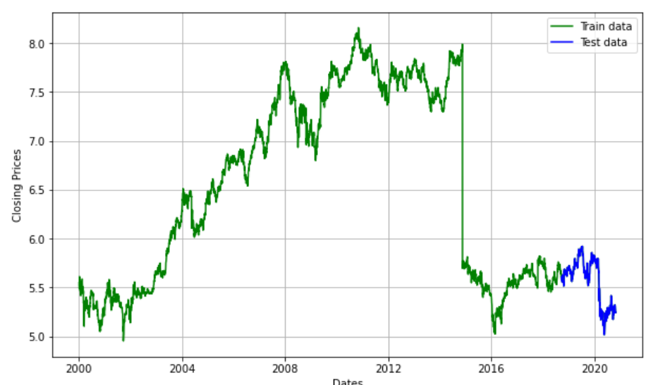
모델을 생성하고 데이터를 Test 와 Train 으로 나눈다

train_data, test_data = df_log[3:int(len(df_log)*0.9)], df_log[int(len(df_log)*0.9):]
plt.figure(figsize=(10,6))
plt.grid(True)
plt.xlabel('Dates')
plt.ylabel('Closing Prices')
plt.plot(df_log, 'green', label='Train data')
plt.plot(test_data, 'blue', label='Test data')
plt.legend()

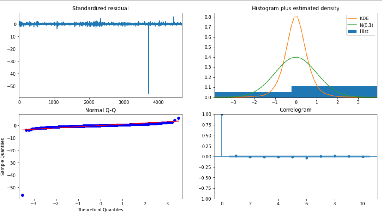
8.AUTO ARIMA 를 통한 최적의 값 탐색

model_autoARIMA = auto_arima(train_data, start_p=0, start_q=0,

test='adf', # use adftest to find optimal 'd'

max_p=3, max_q=3, # maximum p and q

m=1, # frequency of series

d=None, # let model determine 'd'

seasonal=False, # No Seasonality

start_P=0,

D=0,

trace=True,

error_action='ignore',

suppress_warnings=True,

stepwise=True)

print(model_autoARIMA.summary()) 

**MODEL 의 반환값은 Dictionary 로 되어있어서 key를 입력시 자동으로 사용가능**

model_autoARIMA.plot_diagnostics(figsize=(15,8))
plt.show()

model = ARIMA(train_data, order=(0, 1, 0))
fitted = model.fit(disp=-1)
print(fitted.summary())

 

**Best ARIMA order 값을 통한 연산**

8.Forecast

fc, se, conf = fitted.forecast(519, alpha=0.05) # 95% confidence

**95% 신뢰도를 설정한다**

fc_series = pd.Series(fc, index=test_data.index)

lower_series = pd.Series(conf[:, 0], index=test_data.index)

upper_series = pd.Series(conf[:, 1], index=test_data.index)

plt.figure(figsize=(12,5), dpi=100)

plt.plot(train_data, label='training')

plt.plot(test_data, color = 'blue', label='Actual Stock Price')

plt.plot(fc_series, color = 'orange',label='Predicted Stock Price')

plt.fill_between(lower_series.index, lower_series, upper_series,color='k', alpha=.10)

plt.title('SBIN Stock Price Prediction')

plt.xlabel('Time')

plt.ylabel('Actual Stock Price')

plt.legend(loc='upper left', fontsize=8)

plt.show()

주의점

예측추세 - 주황색 - 데이터 값의 index 는 test data의 index를 시작으로함

데이터의 크기 = index의 수 = 예측을 위한 날짜수 가 일치해야함